VeloDB Cloud Quick Start
This guide walks you through getting started with VeloDB Cloud in minutes. You'll create a warehouse, load a 6-million-row SSB-Flat benchmark dataset, and run analytical queries.
No credit card required. VeloDB Cloud offers a 14-day free trial for SaaS warehouses.
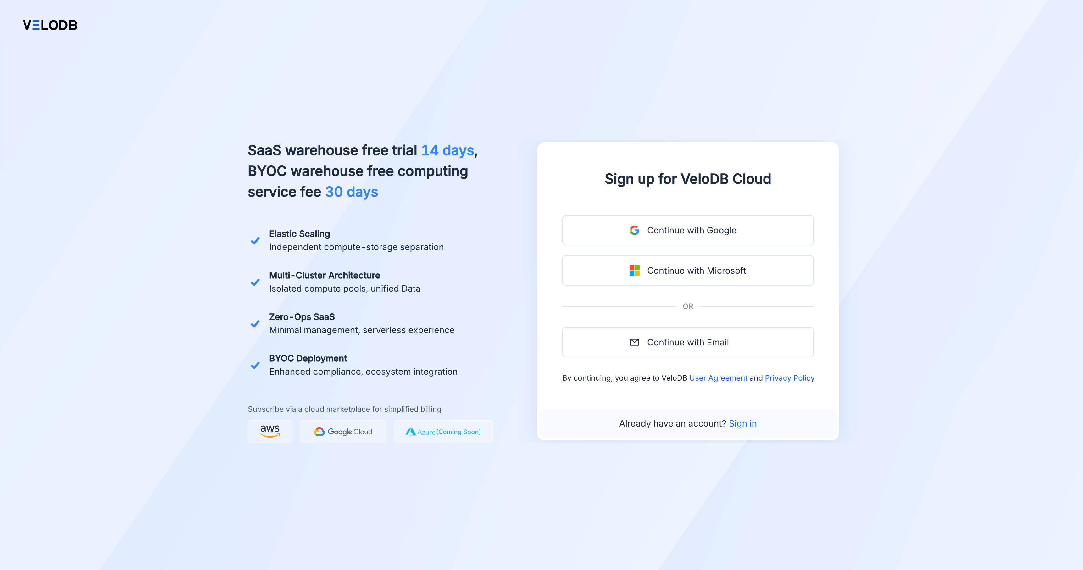
1. Create Your Account
Go to velodb.cloud and sign up using your preferred method:
- Google - Single sign-on with your Google account
- Microsoft - Single sign-on with your Microsoft account
- Email - Traditional email and password registration
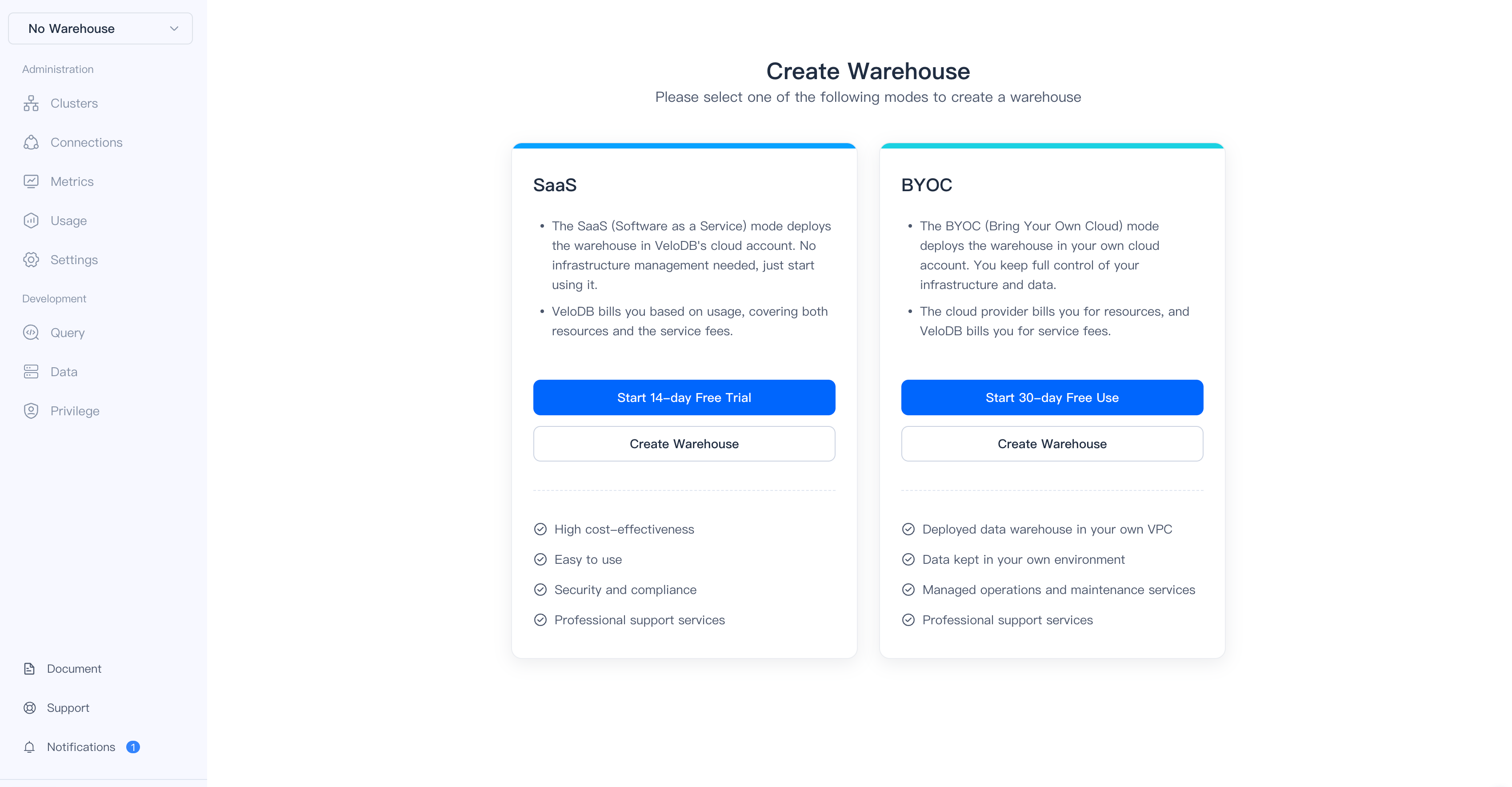
2. Choose Your Deployment Mode
After signing in, you'll see two deployment options:
| Mode | Description | Free Trial |
|---|---|---|
| SaaS | Fully managed warehouse in VeloDB's cloud | 14 days |
| BYOC | Deploy in your own AWS/Azure account | 30 days free service |
For this quickstart, click Start 14-day Free Trial under SaaS.
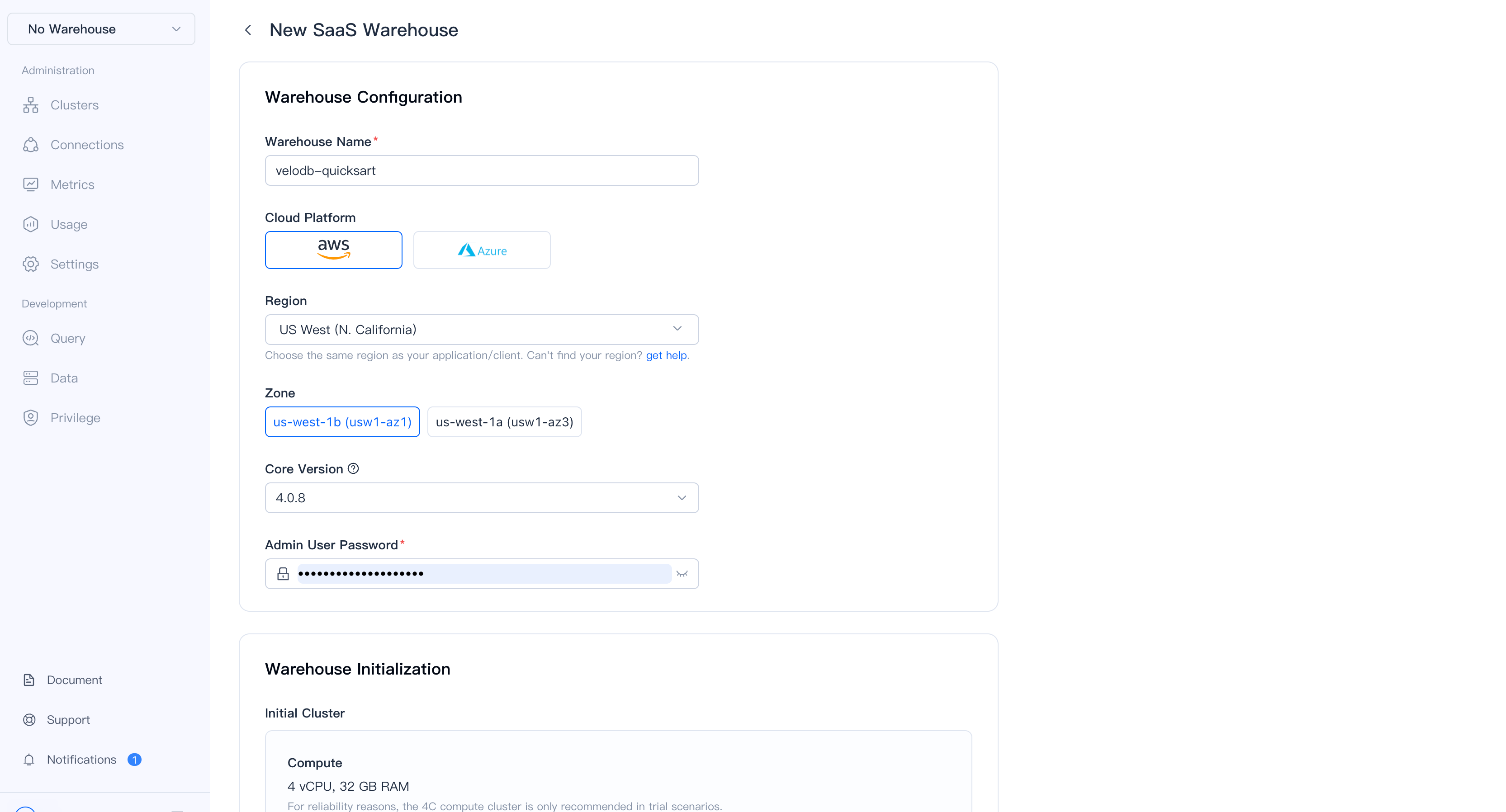
3. Create Your Warehouse
Configure your warehouse with these settings:
| Setting | Recommended Value |
|---|---|
| Warehouse Name | velodb-quickstart |
| Cloud Platform | AWS |
| Region | Select the region closest to you |
| Zone | Any available zone |
| Admin Password | Your secure password |
Important: Remember your admin password. You'll need it to connect to the warehouse.
The initial cluster comes with:
- 4 vCPU, 32 GB RAM compute
- 200 GB cache storage
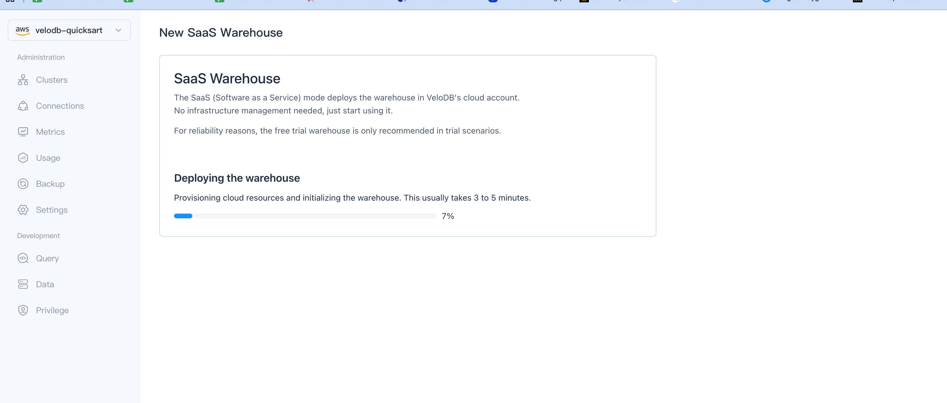
Click Create to provision your warehouse.
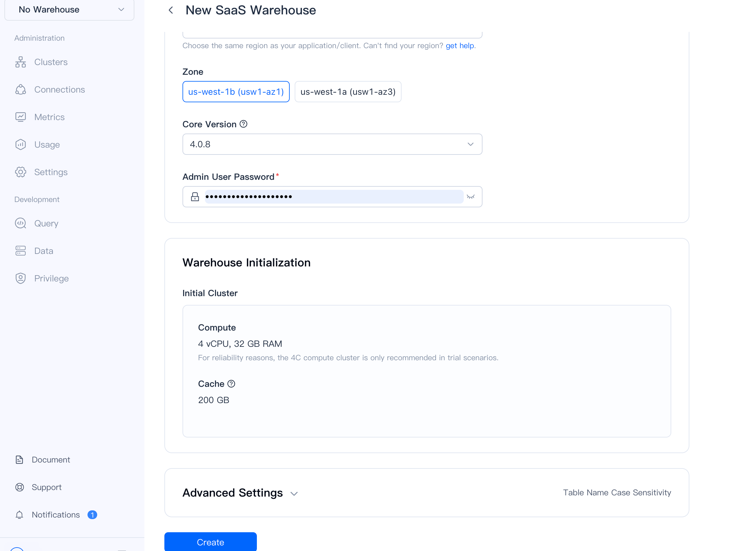
VeloDB provisions your warehouse in 3-5 minutes. Once complete, the status changes to Running.
4. Connect to Your Warehouse
Navigate to Connections in the sidebar to find your connection details:
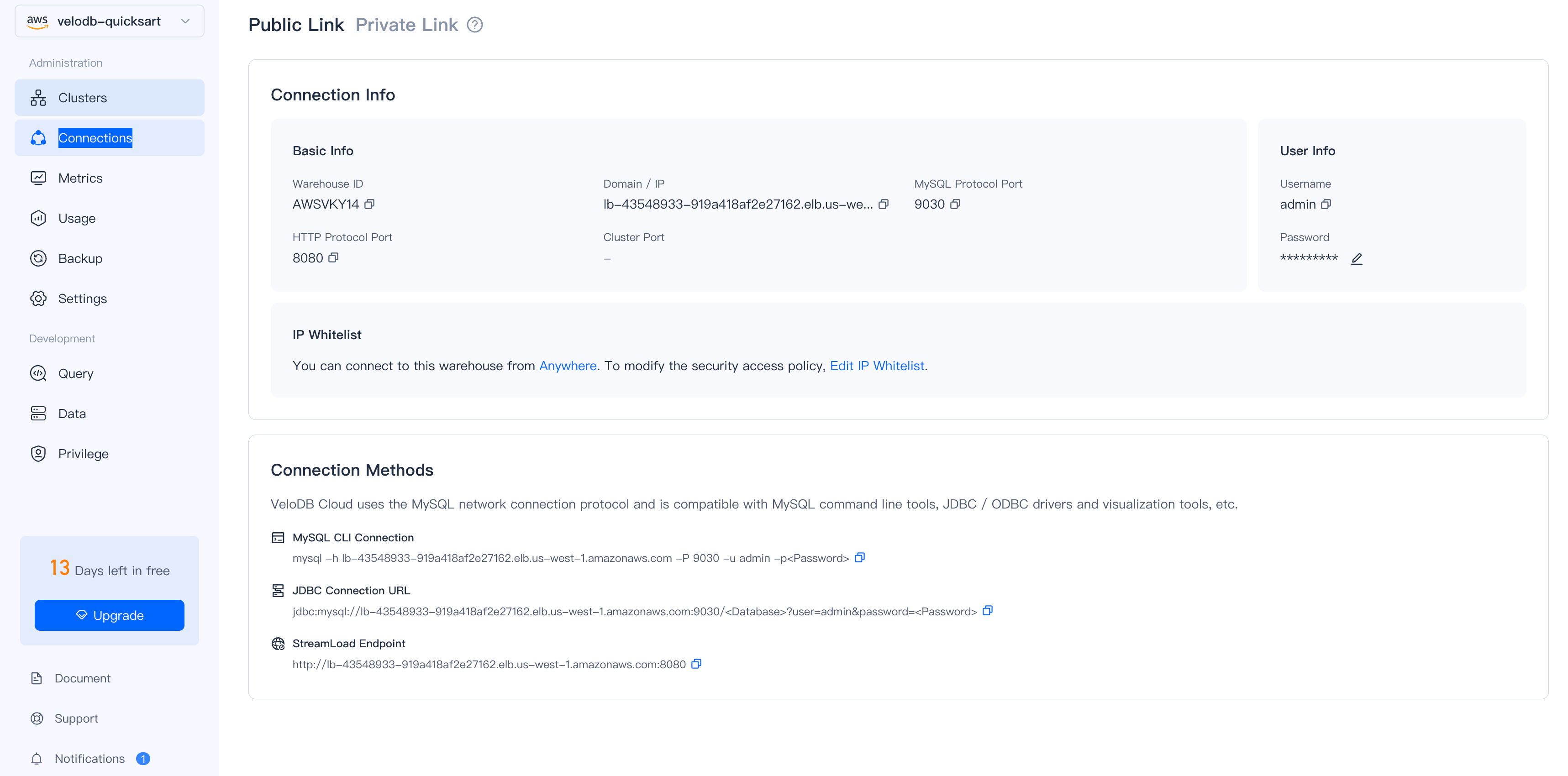
Connection Methods
- SQL Console (Recommended)
- MySQL CLI
- JDBC
Use the built-in Query editor in the VeloDB Console sidebar for browser-based SQL access. No setup required.
mysql -h <your-host>.elb.<region>.amazonaws.com -P 9030 -u admin -p
jdbc:mysql://<your-host>.elb.<region>.amazonaws.com:9030/<database>
Verify Connection
SHOW DATABASES;
Expected output:
+--------------------+
| Database           |
+--------------------+
| information_schema |
+--------------------+
5. Load the SSB-Flat Benchmark Dataset
We've prepared a public SSB-Flat SF1 dataset (6 million rows) for you to explore. This denormalized Star Schema Benchmark dataset is ideal for analytical queries.
No credentials needed! The sample data buckets are publicly accessible from VeloDB.
Preview Data from S3
Before loading, preview the data directly from S3. Select the tab matching your warehouse region for best performance:
- US East (N. Virginia)
- US West (N. California)
- US West (Oregon)
- EU (Frankfurt)
- EU (Ireland)
- Asia Pacific (Singapore)
- Asia Pacific (Tokyo)
- Middle East (Bahrain)
SELECT
    lo_orderkey,
    lo_orderdate,
    c_name,
    c_nation,
    lo_revenue,
    p_brand
FROM S3(
    "uri" = "s3://velodb-import-data-us-east-1/ssb-flat-sf1/ssb_flat_001.parquet",
    "format" = "parquet",
    "s3.endpoint" = "s3.us-east-1.amazonaws.com",
    "s3.region" = "us-east-1"
)
LIMIT 5;
SELECT
    lo_orderkey,
    lo_orderdate,
    c_name,
    c_nation,
    lo_revenue,
    p_brand
FROM S3(
    "uri" = "s3://velodb-import-data-us-west-1/ssb-flat-sf1/ssb_flat_001.parquet",
    "format" = "parquet",
    "s3.endpoint" = "s3.us-west-1.amazonaws.com",
    "s3.region" = "us-west-1"
)
LIMIT 5;
SELECT
    lo_orderkey,
    lo_orderdate,
    c_name,
    c_nation,
    lo_revenue,
    p_brand
FROM S3(
    "uri" = "s3://velodb-import-data-us-west-2/ssb-flat-sf1/ssb_flat_001.parquet",
    "format" = "parquet",
    "s3.endpoint" = "s3.us-west-2.amazonaws.com",
    "s3.region" = "us-west-2"
)
LIMIT 5;
SELECT
    lo_orderkey,
    lo_orderdate,
    c_name,
    c_nation,
    lo_revenue,
    p_brand
FROM S3(
    "uri" = "s3://velodb-import-data-eu-central-1/ssb-flat-sf1/ssb_flat_001.parquet",
    "format" = "parquet",
    "s3.endpoint" = "s3.eu-central-1.amazonaws.com",
    "s3.region" = "eu-central-1"
)
LIMIT 5;
SELECT
    lo_orderkey,
    lo_orderdate,
    c_name,
    c_nation,
    lo_revenue,
    p_brand
FROM S3(
    "uri" = "s3://velodb-import-data-eu-west-1/ssb-flat-sf1/ssb_flat_001.parquet",
    "format" = "parquet",
    "s3.endpoint" = "s3.eu-west-1.amazonaws.com",
    "s3.region" = "eu-west-1"
)
LIMIT 5;
SELECT
    lo_orderkey,
    lo_orderdate,
    c_name,
    c_nation,
    lo_revenue,
    p_brand
FROM S3(
    "uri" = "s3://velodb-import-data-ap-southeast-1/ssb-flat-sf1/ssb_flat_001.parquet",
    "format" = "parquet",
    "s3.endpoint" = "s3.ap-southeast-1.amazonaws.com",
    "s3.region" = "ap-southeast-1"
)
LIMIT 5;
SELECT
    lo_orderkey,
    lo_orderdate,
    c_name,
    c_nation,
    lo_revenue,
    p_brand
FROM S3(
    "uri" = "s3://velodb-import-data-ap-northeast-1/ssb-flat-sf1/ssb_flat_001.parquet",
    "format" = "parquet",
    "s3.endpoint" = "s3.ap-northeast-1.amazonaws.com",
    "s3.region" = "ap-northeast-1"
)
LIMIT 5;
SELECT
    lo_orderkey,
    lo_orderdate,
    c_name,
    c_nation,
    lo_revenue,
    p_brand
FROM S3(
    "uri" = "s3://velodb-import-data-me-south-1/ssb-flat-sf1/ssb_flat_001.parquet",
    "format" = "parquet",
    "s3.endpoint" = "s3.me-south-1.amazonaws.com",
    "s3.region" = "me-south-1"
)
LIMIT 5;
Create Database and Table
-- Create database
CREATE DATABASE IF NOT EXISTS ssb;
USE ssb;

-- Create the SSB flat table
CREATE TABLE IF NOT EXISTS ssb_flat (
    lo_orderkey        BIGINT NOT NULL,
    lo_linenumber      BIGINT NOT NULL,
    lo_custkey         BIGINT NOT NULL,
    lo_partkey         BIGINT NOT NULL,
    lo_suppkey         BIGINT NOT NULL,
    lo_orderdate       DATE NOT NULL,
    lo_commitdate      DATE NOT NULL,
    lo_orderpriority   VARCHAR(15) NOT NULL,
    lo_shippriority    BIGINT NOT NULL,
    lo_shipmode        VARCHAR(10) NOT NULL,
    lo_year            INT NOT NULL,
    lo_month           INT NOT NULL,
    lo_weeknum         INT NOT NULL,
    d_datekey          BIGINT NOT NULL,
    d_dayofweek        VARCHAR(10) NOT NULL,
    d_month            VARCHAR(10) NOT NULL,
    d_yearmonth        VARCHAR(10) NOT NULL,
    lo_quantity        BIGINT NOT NULL,
    lo_extendedprice   DOUBLE NOT NULL,
    lo_discount        DOUBLE NOT NULL,
    lo_revenue         DOUBLE NOT NULL,
    lo_supplycost      DOUBLE NOT NULL,
    lo_tax             DOUBLE NOT NULL,
    c_custkey          BIGINT NOT NULL,
    c_name             VARCHAR(25) NOT NULL,
    c_nation           VARCHAR(15) NOT NULL,
    c_region           VARCHAR(12) NOT NULL,
    c_city             VARCHAR(10) NOT NULL,
    c_mktsegment       VARCHAR(10) NOT NULL,
    s_suppkey          BIGINT NOT NULL,
    s_name             VARCHAR(25) NOT NULL,
    s_nation           VARCHAR(15) NOT NULL,
    s_region           VARCHAR(12) NOT NULL,
    s_city             VARCHAR(10) NOT NULL,
    p_partkey          BIGINT NOT NULL,
    p_name             VARCHAR(22) NOT NULL,
    p_brand            VARCHAR(9) NOT NULL,
    p_category         VARCHAR(7) NOT NULL,
    p_mfgr             VARCHAR(6) NOT NULL,
    p_color            VARCHAR(11) NOT NULL,
    p_type             VARCHAR(25) NOT NULL,
    p_size             BIGINT NOT NULL,
    p_container        VARCHAR(10) NOT NULL,
    INDEX idx_p_type (p_type) USING INVERTED PROPERTIES("parser" = "english")
)
DUPLICATE KEY(lo_orderkey)
DISTRIBUTED BY HASH(lo_orderkey) BUCKETS 48;
Load Data
For best performance, use the S3 bucket in the same region as your warehouse.
- US East (N. Virginia)
- US West (N. California)
- US West (Oregon)
- EU (Frankfurt)
- EU (Ireland)
- Asia Pacific (Singapore)
- Asia Pacific (Tokyo)
- Middle East (Bahrain)
INSERT INTO ssb.ssb_flat
SELECT * FROM S3(
    "uri" = "s3://velodb-import-data-us-east-1/ssb-flat-sf1/*.parquet",
    "format" = "parquet",
    "s3.endpoint" = "s3.us-east-1.amazonaws.com",
    "s3.region" = "us-east-1"
);
INSERT INTO ssb.ssb_flat
SELECT * FROM S3(
    "uri" = "s3://velodb-import-data-us-west-1/ssb-flat-sf1/*.parquet",
    "format" = "parquet",
    "s3.endpoint" = "s3.us-west-1.amazonaws.com",
    "s3.region" = "us-west-1"
);
INSERT INTO ssb.ssb_flat
SELECT * FROM S3(
    "uri" = "s3://velodb-import-data-us-west-2/ssb-flat-sf1/*.parquet",
    "format" = "parquet",
    "s3.endpoint" = "s3.us-west-2.amazonaws.com",
    "s3.region" = "us-west-2"
);
INSERT INTO ssb.ssb_flat
SELECT * FROM S3(
    "uri" = "s3://velodb-import-data-eu-central-1/ssb-flat-sf1/*.parquet",
    "format" = "parquet",
    "s3.endpoint" = "s3.eu-central-1.amazonaws.com",
    "s3.region" = "eu-central-1"
);
INSERT INTO ssb.ssb_flat
SELECT * FROM S3(
    "uri" = "s3://velodb-import-data-eu-west-1/ssb-flat-sf1/*.parquet",
    "format" = "parquet",
    "s3.endpoint" = "s3.eu-west-1.amazonaws.com",
    "s3.region" = "eu-west-1"
);
INSERT INTO ssb.ssb_flat
SELECT * FROM S3(
    "uri" = "s3://velodb-import-data-ap-southeast-1/ssb-flat-sf1/*.parquet",
    "format" = "parquet",
    "s3.endpoint" = "s3.ap-southeast-1.amazonaws.com",
    "s3.region" = "ap-southeast-1"
);
INSERT INTO ssb.ssb_flat
SELECT * FROM S3(
    "uri" = "s3://velodb-import-data-ap-northeast-1/ssb-flat-sf1/*.parquet",
    "format" = "parquet",
    "s3.endpoint" = "s3.ap-northeast-1.amazonaws.com",
    "s3.region" = "ap-northeast-1"
);
INSERT INTO ssb.ssb_flat
SELECT * FROM S3(
    "uri" = "s3://velodb-import-data-me-south-1/ssb-flat-sf1/*.parquet",
    "format" = "parquet",
    "s3.endpoint" = "s3.me-south-1.amazonaws.com",
    "s3.region" = "me-south-1"
);
Loading 6 million rows takes approximately 30 seconds to 1 minute.
Verify Load
SELECT COUNT(*) AS total_rows FROM ssb.ssb_flat;
Expected output:
+------------+
| total_rows |
+------------+
|    6000000 |
+------------+
6. Run Analytical Queries
Now let's run some analytical queries on your dataset.
Query 1: Real-Time Aggregation
Aggregate revenue and discount metrics by customer region:
SELECT
    c_region,
    COUNT(*) AS order_count,
    SUM(lo_revenue) AS total_revenue,
    AVG(lo_discount) AS avg_discount
FROM ssb.ssb_flat
GROUP BY c_region
ORDER BY total_revenue DESC;
Query 2: Window Functions - YoY Growth
Calculate year-over-year revenue growth using window functions:
SELECT
    lo_year,
    SUM(lo_revenue) AS yearly_revenue,
    LAG(SUM(lo_revenue)) OVER (ORDER BY lo_year) AS prev_year_revenue,
    ROUND(
        (SUM(lo_revenue) - LAG(SUM(lo_revenue)) OVER (ORDER BY lo_year))
        / LAG(SUM(lo_revenue)) OVER (ORDER BY lo_year) * 100,
        2
    ) AS yoy_growth_pct
FROM ssb.ssb_flat
GROUP BY lo_year
ORDER BY lo_year;
Query 3: Complex BI with CTE
Use Common Table Expressions to analyze regional profit tiers:
WITH regional_stats AS (
    SELECT
        c_region,
        s_region,
        SUM(lo_revenue) AS revenue,
        SUM(lo_supplycost) AS cost,
        SUM(lo_revenue - lo_supplycost) AS profit
    FROM ssb.ssb_flat
    GROUP BY c_region, s_region
)
SELECT
    c_region,
    s_region,
    revenue,
    profit,
    CASE
        WHEN profit > 1000000000 THEN 'High'
        WHEN profit > 500000000 THEN 'Medium'
        ELSE 'Low'
    END AS profit_tier
FROM regional_stats
ORDER BY profit DESC;
Query 4: Self-Join Period Comparison
Compare revenue between 1997 and 1993 using a self-join:
SELECT
    t1.c_nation,
    t1.revenue_1997,
    t2.revenue_1993,
    ROUND((t1.revenue_1997 - t2.revenue_1993) / t2.revenue_1993 * 100, 2) AS growth_pct
FROM (
    SELECT c_nation, SUM(lo_revenue) AS revenue_1997
    FROM ssb.ssb_flat
    WHERE lo_year = 1997
    GROUP BY c_nation
) t1
JOIN (
    SELECT c_nation, SUM(lo_revenue) AS revenue_1993
    FROM ssb.ssb_flat
    WHERE lo_year = 1993
    GROUP BY c_nation
) t2 ON t1.c_nation = t2.c_nation
ORDER BY growth_pct DESC;
Query 5: Full-Text Search
Search for products containing "STEEL" in the product type using inverted index:
SELECT
    p_type,
    p_brand,
    COUNT(*) AS product_count,
    SUM(lo_revenue) AS total_revenue
FROM ssb.ssb_flat
WHERE p_type MATCH 'STEEL'
GROUP BY p_type, p_brand
ORDER BY total_revenue DESC
LIMIT 10;
Next Steps
- Set up billing - Add a payment method via the Billing Center
- Import your own data - See the S3 Import Guide
- Learn more - Explore the VeloDB documentation