Vector Quantization Survey and Selection Guide

This document introduces common vector quantization methods from a practical perspective, and explains how to apply them in VeloDB Cloud ANN workloads.

Why Quantization Is Needed

For ANN workloads, especially HNSW, index memory can quickly become the bottleneck. Quantization maps high-precision vectors (usually float32) to lower-precision codes, trading a small amount of recall for lower memory usage.

In VeloDB Cloud, quantization is controlled by the quantizer property in ANN indexes:

• flat: no quantization (highest quality, highest memory)
• sq8: scalar quantization, 8-bit
• sq4: scalar quantization, 4-bit
• pq: product quantization

Example (HNSW + quantizer):

CREATE TABLE vector_tbl (
  id BIGINT,
  embedding ARRAY<FLOAT>,
  INDEX ann_idx (embedding) USING ANN PROPERTIES (
    "index_type" = "hnsw",
    "metric_type" = "l2_distance",
    "dim" = "768",
    "quantizer" = "sq8"
  )
)
DUPLICATE KEY(id)
DISTRIBUTED BY HASH(id) BUCKETS 8
PROPERTIES ("replication_num" = "3");

Method Overview

Method	Core Idea	Typical Gain	Main Cost
SQ (Scalar Quantization)	Quantize each dimension independently	Large memory reduction, simple implementation	Build slower than FLAT; recall drops with stronger compression
PQ (Product Quantization)	Split vector into subvectors, quantize each subvector with codebooks	Better compression/latency balance on many datasets	Training/encoding cost is high; tuning is required

VeloDB Cloud currently uses an optimized Faiss implementation as the core engine for ANN vector indexing and search. The SQ/PQ behavior discussed below is therefore directly relevant to VeloDB Cloud in practice.

Scalar Quantization (SQ)

Principle

SQ keeps the vector dimension unchanged and only lowers per-dimension precision.

A standard min-max mapping per dimension is:

• max_code = (1 << b) - 1
• scale = (max_val - min_val) / max_code
• code = round((x - min_val) / scale)

Faiss SQ has two styles:

• Uniform: all dimensions share one min/max range.
• Non-uniform: each dimension uses its own min/max.

When dimensions have very different value ranges, non-uniform SQ usually gives better reconstruction quality.

Key Characteristics

• Strengths:
  • Straightforward and stable.
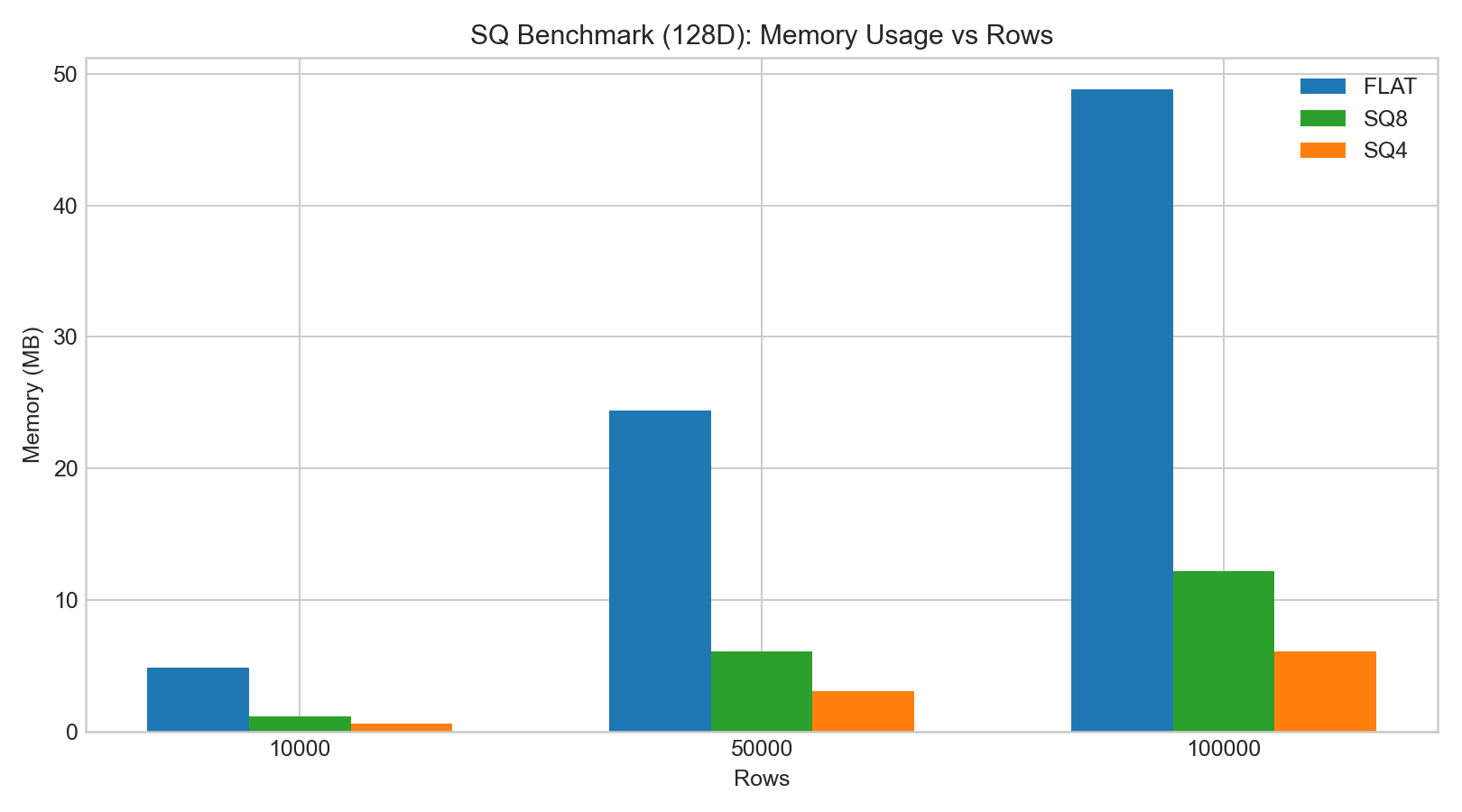
  • Predictable compression (sq8 roughly 4x vs float32 values, sq4 roughly 8x).
• Weaknesses:
  • Assumes distribution can be bucketed with fixed steps.
  • If a dimension is highly non-uniform (for example, strong long-tail), quantization error can increase.

Faiss Source-Level Note (SQ)

Under the VeloDB Cloud + optimized Faiss implementation path, SQ training computes min/max statistics first, then expands the range slightly to reduce out-of-range risk at add time. A simplified shape is:

void train_Uniform(..., const float* x, std::vector<float>& trained) {
    trained.resize(2);
    float& vmin = trained[0];
    float& vmax = trained[1];
    // scan all values to get min/max
    // then optionally expand range by rs_arg
}

For non-uniform SQ, Faiss computes statistics per dimension (instead of one global range), which is why it typically behaves better when different dimensions have very different value scales.

Practical Observations

In the internal 128D/256D HNSW tests:

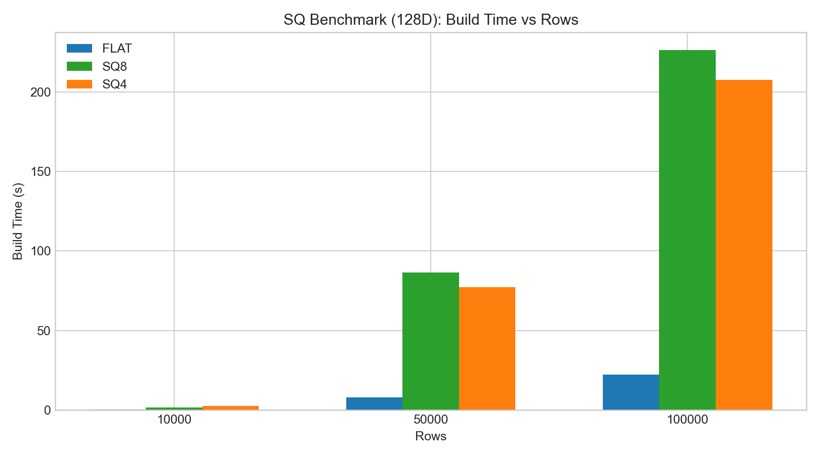
• sq8 generally preserved recall better than sq4.
• SQ index build/add time was significantly higher than FLAT.
• Search latency change was often small for sq8, while sq4 had larger recall drop.

The following bar charts are based on example benchmark data:

Product Quantization (PQ)

Principle

PQ splits a D-dim vector into M subvectors (D/M dimensions each), then applies k-means codebooks to each subspace.

Main parameters:

• pq_m: number of subquantizers (subvectors)
• pq_nbits: bits per subvector code

Larger pq_m usually improves quality but increases training/encoding cost.

Why PQ Can Be Faster at Query Time

PQ can use LUT (look-up table) distance estimation:

• Precompute distances between query subvectors and codebook centroids.
• Approximate full-vector distance by table lookups + accumulation.

This avoids full reconstruction and can reduce search CPU cost.

Faiss Source-Level Note (PQ)

Under the same implementation path, Faiss ProductQuantizer trains codebooks over subspaces and stores them in a contiguous centroid table. A simplified shape is:

void ProductQuantizer::train(size_t n, const float* x) {
    Clustering clus(dsub, ksub, cp);
    IndexFlatL2 index(dsub);
    clus.train(n * M, x, index);
    for (int m = 0; m < M; m++) {
        set_params(clus.centroids.data(), m);
    }
}

Centroids are laid out as (M, ksub, dsub), where:

• M: number of subquantizers,
• ksub: codebook size per subspace (2^pq_nbits),
• dsub: subvector dimension (D / M).

Practical Observations

In the same internal tests:

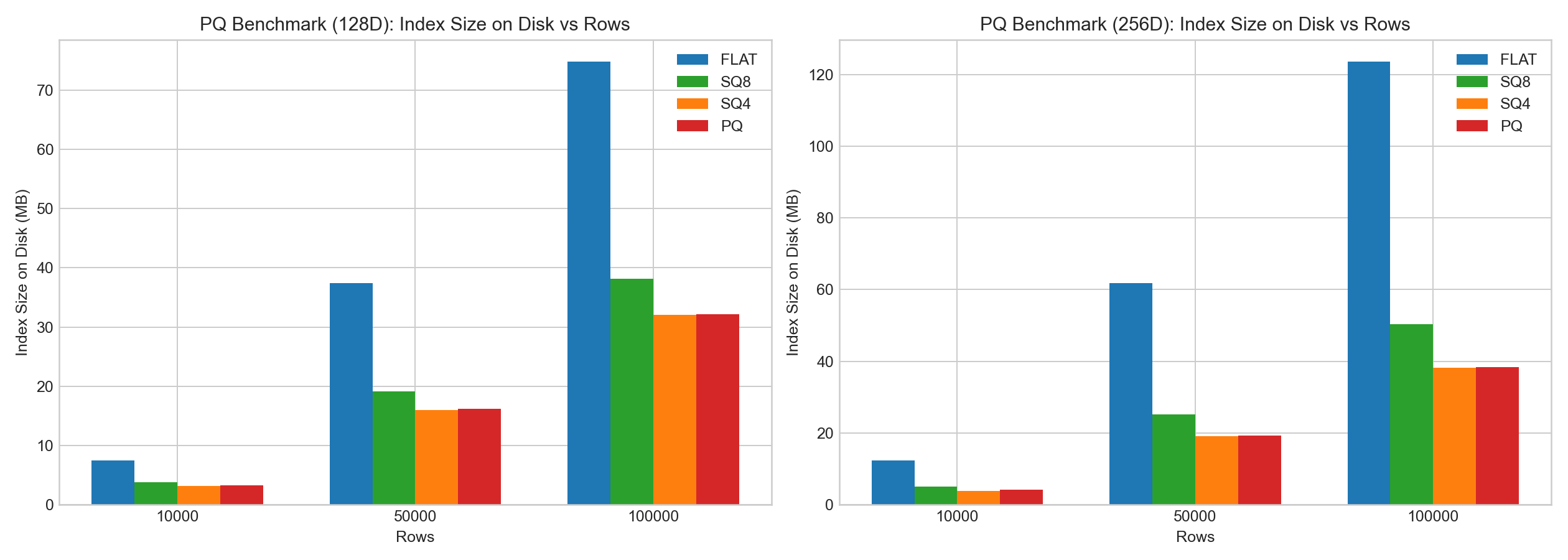
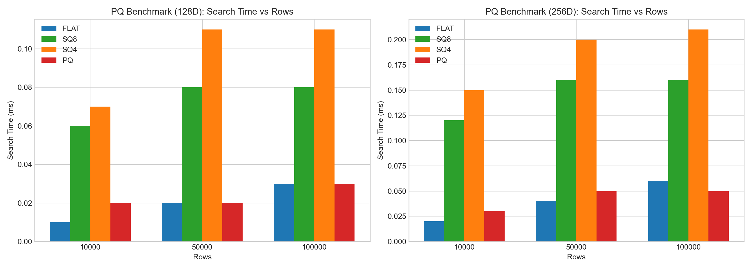
• PQ showed clear compression benefits.
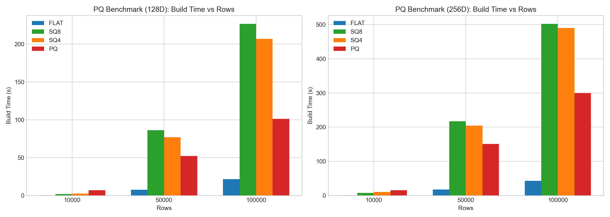
• PQ encoding/training overhead was high.
• Compared with SQ, PQ often had better search-time behavior due to LUT acceleration, but recall/build trade-offs depended on data and parameters.

The following bar charts are based on example benchmark data:

Practical Selection Guide for VeloDB Cloud

Use this as a starting point:

1. Memory is sufficient and recall is top priority: flat.
2. Need low risk compression with relatively stable quality: sq8.
3. Extreme memory pressure and can accept lower recall: sq4.
4. Need stronger memory-performance balance and can spend time tuning: pq.

Recommended validation process:

1. Start with flat as baseline.
2. Test sq8 first; compare recall and P95/P99 latency.
3. If memory is still too high, test pq (pq_m = D/2 as first trial).
4. Use sq4 only when memory reduction has higher priority than recall.

Benchmarking Notes

• Absolute times are hardware/thread/dataset dependent.
• Compare methods under the same:
  • vector dimension,
  • index parameters,
  • segment size,
  • query set and ground truth.
• Evaluate both quality and cost:
  • Recall@K,
  • index size,
  • build time,
  • query latency.

Related Documents

• Overview
• HNSW
• IVF
• ANN Resource Estimation Guide